Astronomy/JS9

A photo of Cassiopeia A (CAS-A) from the Chandra X-Ray Observatory viewed in the JS9 interface, showing various controls and the color map

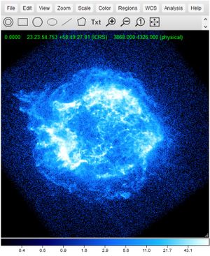
JS9 is a web-based astronomical image analysis software. It was first introduced in the 2020 season to add a hands-on component to Astronomy. With event supervisor permission, teams will be able to access the internet to answer sections involving this software. The JS9 website specifically made for Science Olympiad can be found at js9.si.edu/nso/nso.html.

Introduction to Image Analysis

Any time we take data with a telescope, we are actually making a record of the light that hits it. This is essentially what you find in a FITS file: a record of all of the light that hit a telescope over a certain period of time. FITS stands for Flexible Image Transport System, and is a file type used for storing astronomical data. Like the images we are used to, a FITS file shows where light hits a detector, and in what intensity. In other words, it can show how much light hit a certain location over a certain amount of time.

However, unlike the images we are used to seeing, FITS files can store other data as well. For example, when the Chandra X-Ray Observatory makes an observation, it is "hit" with a series of photons (or light particles) from wherever it is looking. The detector is able to determine where the photon hit the detector (position), when the photon hit the detector (time), and how much energy the photon had when it hit the detector (energy). It then records all three of these things into a FITS file.

The purpose of Image Analysis (or Image Processing) software is to be able to decode these FITS files and perform some sort of data analysis on them. For example, if we know when and where light hits the detector, then we can generate a light curve (a plot of how much light hit the detector over a period of time) of a certain area of the detector. JS9 serves as the platform that we can use to both view the FITS data, and to perform different analysis functions on it.

Opening Files

The File Menu

The JS9 software opens FITS files (files with the *.fits extension). Most files that will be used for JS9 questions will use the *_evt2.fits extension, which includes X-Ray event data. Files can be opened locally or remotely, or you can open the example files on the NSO JS9 page.

Open Example

When the JS9 site specifically developed for Science Olympiad is opened, there are six example links at the top of the site. Selecting one of these links will open one of the example images. These images are good to start with when first working with JS9 because they are good images, and you won't have to sort through a lot of images that aren't easily analyzable to find them.

Open Local

In the File > Open Local menu, you can upload and open a downloaded FITS file.

Open Remote

In the File > Open Remote menu, you can use a proxy or CORS server to open a FITS file remotely from a link.

Proxy Server

When this is selected, you can open a file from a link that does not support CORS (Cross-Origin Resource Sharing), such as the Unofficial Chandra Archive. This will not display directly in JS9, but JS9 servers will retrieve the information to display the file. This option is the most commonly used, as it allows for a wide variety of links directly from archives.

CORS Server

This option will directly retrieve the image from a site that supports CORS (such as dropbox) and display the image directly in JS9.

Finding FITS Files

A great way to learn JS9 is to practice with JS9. For starting, you might want to start with the six files at the top of the JS9 interface, as those files are excellent, and you don't have to go looking for them. Many telescopes have a large archive of data that they have collected in the past, and these can be an excellent source for FITS files. The most commonly used data is from NASA's Chandra X-Ray Observatory, although data from other telescopes have also been used in the past.

The UnOfficial Chandra Archive

The UnOfficial Chandra Archive (The Unofficial Chandra Archive) is the easiest and most common place to get FITS files for a JS9 analysis. In comparison to other archives, it is easy to search for and get a link to open a file, and the Chandra X-Ray Center data is very useful for analysis. It contains quite a few objects, including many of the DSOs.

First, you will need to search for an image.

• If you have the Observation ID of an image (most Chandra Photo Album articles have an Observation ID at the bottom that tells you what FITS file was used to generate the image), you can enter that in the ObsID field, and search for the image.
• If you know the name of the object that you want to search for, you can enter that in the "Name" field. This will give you a list of all of the FITS files for objects within a certain range (default of 30′) from the object you specified.
  • Troubleshooting: If the name you specified resulted in "Cannot lookup name...", it means that they have the object under a different name. You can search the object name you have and try to find alternate object names (most Wikipedia pages about objects have alternative names for them).
  • Troubleshooting: If the name you specified resulted in "Search Results : Found 0 Matches", then the Chandra Archive does not contain the object you searched for.
• If you have the coordinates of the object, you can use the "RA" and "Dec" fields. Enter the Right Ascension in the RA field, in the form h:mm:ss.ss (for example, if the right ascension is 12h 29m 06.7s, you would enter 12:29:06.7). Then enter the Declination in the Dec field in the form ±dd:mm:ss.ss (for example, if the declination is +02° 03′ 09″, you would enter +02:03:09).
• If you know what type of object you want to observe, but don't have a specific object, you can search the "Title Key" field. This will search the proposal titles of all FITS files and list any files that have your search term in their name. For example, if I wanted to look at objects with Radio Lobes, I could enter "Radio Lobe" in the Title Key field.

Next, you will have to pick an image out of the list. You can take a look at the proposal titles to find out what each observer was specifically looking for, and you can use the "Exposure" column. This tells you how long the telescope looked at the object in kiloseconds. As a general rule of thumb, the higher the exposure, the better your light analysis of the object will be (that is, the energy spectrum, light curve, etc. of the object). Images with an exposure of less than 20ks generally aren't observed for long enough to easily discern the object, and analysis tends to be noisy. An exposure of too high (generally over 100, although this is heavily dependent on the object) will probably get you an excellent light analysis of the object, but you probably won't be able to see much of the object itself, it will just appear as a bright circle. In addition to exposure, there are a lot of different factors that influence images, so try a few out until you find what you like.

The final step to getting an image from the UnOfficial Chandra Archive is to get the link. To do this, click on the Observation ID of the image you would like to open, find the link that ends in *evt2.fits (or any other link for that matter, the X-Ray event file is generally the most useful, though). Right click on this link and copy the link location. Now, you can simply use the "Open Remote" function described above to open this link.

Alternative Chandra Data Archive

The UnOfficial Chandra Archive above has the easiest interface for finding FITS files, but does not get updated and is notorious for going down at random times. If it does, you can still obtain FITS files taken by Chandra another way, you just need the observation ID of the file first.

If you know the object that you want to search for (or the coordinates of the object), you can search the Chandra Footprint Service. You can then get the observation ID of any data file from the ObsID Column (the leftmost column by default).

Once you have the observation ID of an object, paste the following link into your browser, replacing LASTDIGIT with the last digit of your observation ID (for example, for an observation ID of 5672, you would replace "LASTDIGIT" with "2"), and OBSID with your observation ID.

https://cxc.cfa.harvard.edu/cdaftp/byobsid/LASTDIGIT/OBSID/primary/

Now, copy the location of the link ending in evt2.fits and open it remotely with JS9. This is the link to the X-Ray event file, which is the most useful file for analyzing X-Ray data, as it contains the most information about the object.

Other Data Archives

If you are interested in analyzing data that is in wavelengths other than X-Ray, you can look at archives from other telescopes. Certain archives may have FITS files that can't be opened by JS9, or other non-FITS data files. Many of these files also do not contain the as much information as an x-ray event file, and so you won't be able to analyze them as deeply.

Here's a list of archives from other telescopes that you can get FITS files from:

• NRAO Science Data Archive (Wavelength: Radio)
  • You can search for an object in this archive, select the images that you want to open in JS9, and get a temporary link to the file sent to an email of your choice.
  • When looking through the images, only the .uvfits can be opened by JS9.
  • The only analysis you can do on this file is "Counts in Regions". That said, you can still make measurements and look at the object, so it is still useful.

Viewing the Image

Zoom

Using the bar at the top, you can click on either of the magnifying glass icons to zoom in or out. Additionally, you can open the "Zoom" menu to get more options on zooming in or out on parts of your image.

Panning

JS9 Panner Window

In the "View" menu of JS9, select the "Panner" option. A separate window will appear that contains a small version of the image with a box around the current area you are viewing. Drag this box anywhere in this small version of the image to pan around the JS9 image. Alternatively, if you are using a mouse, you can right-click and drag to pan around the image.

Colormaps

JS9 displays images in false color based on data. In the "Color" menu, you will be given a dropdown of different color schemes to change the colormap of your image. This changes how different intensities of the image appear. Playing with different colormaps can give you an idea of which one works best for you.

Contrast and Bias

You can adjust the contrast and bias of an image to highlight different parts of the image of different intensities. To adjust the contrast (or make the range over which the color covers change) click on the image and drag your mouse up and down. To adjust the bias (or the intensity over which the contrast is centered), drag the mouse left and right. This can help you determine areas of high intensity, or a certain intensity.

Composite and Overlaid Images

Example RGB overlay using three different images

If you have 2 or 3 images, you can overlay them. This is useful if you have two or three images in different wavelengths of a single object (e.g. created through an energy Event Filter), you can overlay them on top of each other to create a composite image.

1. The first step is to put each image in a red, green, or blue colormap. Only images in these colormaps can be overlaid.
2. Adjust each different image as you see fit. This may require zooming out or panning to make all of them aligned, or adjusting contrast and bias. You can switch between images in the "File" menu.
3. Select "rgb mode" from the "Color" menu to overlay images in the red, green, and blue colormaps on top of each other.

Every measurement done on an image in JS9 will be using a coordinate system. The default coordinate system for JS9 is FK5 (or a system of coordinates where you describe angular position in degrees, arcminutes, and arcseonds in relation to a reference). To change the coordinate system, look through the WCS (standing for World Coordinate System) menu, and select one of the coordinate options. FK4, FK5, and ICRS all show angular position in the sky in degrees, arcminutes, and arcseconds (with different references), where galactic, ecliptic, physical, and image all show the position on the sky in pixels (with different reference points). It can be useful to switch your coordinate system to a system that measures in pixels if you have to make a measurement of the diameter of an object in pixels.

Analysis with the "Analysis" Menu

In this section, we outline how you can make use of the FITS data to gather information about an object.

Performing an analysis in JS9 is rather simple. First, you have to tell the software what part of the file you want to analyze (that is, putting a region around something). Then, you run whatever analysis or combination thereof you need to to obtain the necessary information about the object in question. While it would be in your best interest to be fluent with all of the analysis functions available to you in JS9, it would be particularly beneficial to learn the Counts in Regions, FITS Headers, Energy Spectrum, Light Curve (both versions), Power Spectrum, Period Folding, and Flux in Regions tools.

There are four different categories that analysis functions fall under, Client-Side Analysis, Server-Side Analysis, NSO Analysis, and ImExam Plugins. Client-Side Analysis and ImExam Plugins can be done from a browser, and the FITS file will not need to be uploaded to a JS9 server. NSO Analysis and Server-Side Analysis can only be run if the FITS file is uploaded to a JS9 server. If you use the "Open Remote" function to open your file, or you open an example file, the file should automatically upload to the remote server. However, if you open a file locally, the file doesn't automatically upload for some reason, or you leave for too long and the file gets deleted from the server, you can upload it using Analysis > "upload FITS to make tasks available" or running analysis uploadfits in the JS9 console. Note that if your image timed out and was deleted, you will have to use the JS9 console to re-upload it to the server.

All of the explanations of analysis in this section assume that you are using an FK5 coordinate system. However, other coordinate systems can be used to gain a different understanding of measurements of objects.

Regions

Analysis in JS9 is done through regions in an image. Regions are geometric shapes that can be placed on an image. These regions indicate areas for analysis, or can be used to indicate areas of interest on the image. A region can be sized over an area of an image, and all pixels inside the region will be analyzed using different analysis functions. For example, if I want to find the energy spectrum of a galaxy cluster, I might put a circle or elliptical region around that galaxy cluster before running the corresponding analysis. All analysis functions can be found in the "Analysis" menu, or can be done through the JS9 console. To open the JS9 console, go to View > Console.

Regions also serve another important purpose: measuring tools. If you place a region on the image and resize it so that it exactly lines up with something you want to measure (for example, the distance between two points, or the radius of a circle), you can use the configuration menu to figure out how large the region is, and therefore, you know the angular measurement.

To insert a region, click on the region shape in the toolbar, or open the "Regions" menu and select the region that you would like to insert.

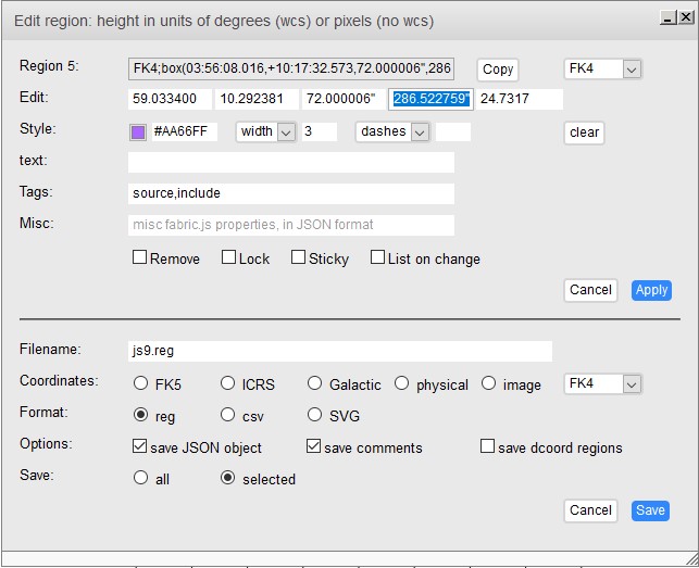
Clicking inside a region will toggle it into focus. You can then move or resize it, as you would a shape in a drawing program. Click outside the region to toggle it out of focus. Double clicking inside a region will open the configuration menu. You can view and change parameters in this menu, and then click apply to save your changes to the region.

Annulus

Default Annulus Configuration Menu

This region is a target-shape. It is considered by many functions as multiple regions, with each space between the lines as its own region. When you insert an annulus, it defaults in the center of your viewing field with two regions. To change the number of regions, double-click on the annulus to bring up the configuration menu. In the third field after the "Edit:" label (this is also the longest of the three fields), there will be three default values, one of them is 0". To add another region, you will need to add another value behind this, which will mark the radius of the next circle out (make sure to insert a comma between all values and quotation marks after each measurement, indicating arcseconds).

Box

This region is rectangular. It defaults as a square, but can be resized as a rectangle. You can manually change the width and height of this region by double-clicking to open the configuration menu and editing the 3rd and 4th boxes after the "Edit" label.

Circle

This region is circular. To change the radius of this region, double-click on it to open the configuration menu. Edit the 3rd text field after the "Edit" label.

Ellipse

This region is elliptical. It defaults as an ellipse with a horizontal radius about 1.5 times the vertical radius, centered on the viewing field. Ellipses can be stretched, compressed, or dilated to the desired shape. Alternatively, the two radii of the ellipse can be entered manually, by double-clicking on the region to open the configuration menu and entering the desired horizontal radius and vertical radius in the 3rd and 4th text fields after the "Edit" label.

Other Regions

The polygon region is a region that defaults to an equilateral triangle centered in the viewing window that can be stretched, compressed, or dilated.

The line region is a linear, one dimensional region. This region analyzes pixels that fall on this line. This line can be adjusted using its endpoints, or selected/moved by clicking on the line.

The point region is a single point region. This analyzes only pixels that fall on that point. This point can be moved or selected by clicking on it.

The text region is not used for analysis, but rather for annotating the image. This may be useful if a test requires you to submit a final image and asks you to indicate a certain point.

Client-Side Analysis

Client-Side Analysis is analysis that can be run in the web browser, and does not require requests to be made to a JS9 server. All functions in this section can be found in the Analysis menu under the grayed-out "Client-side Analysis" heading.

Analysis	Location in Menu	JS9 Console Command	Description/Use	Screenshots
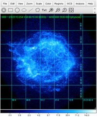
Coordinate Grid	Analysis > Coordinate Grid	N/A	This displays a coordinate grid over the image.	Client-Side Analysis Coordinate Grid
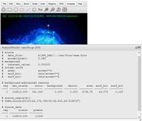
Counts in Regions	Analysis > Counts in Regions Note: This is the one under the Client-side analysis heading.	analysis counts	The main purpose of this function is to count the photons (counts) in all of the regions in the image. However, it also tells you how many arcseconds are in each pixel on the image (arcseconds/pixel) which is a very useful conversion factor for getting between arcseconds and pixels. Additionally, this function give you information about the area of the region(s) you are using.	Counts in Regions Analysis
Radial Profile	Analysis > Radial Profile Note: This is the one under the Client-side analysis heading.	analysis radialprofile	Radial Profile requires an annulus. This determines the flux in each region (in photons/square arcsecond) and plot the value for each region in the annulus on a graph of the surface brightness vs. the radius. This is identical to the Server-side analysis version.	Radial Profile graph. The bump in the center corresponds to the increase in brightness of the image near the bottom-left of the annulus.
Gaussian Blur	Analysis > Blur, equivalent sigma	N/A	This blurs the image pixel values together using a Gaussian function. You will specify a radius (sigma) in the text field and the pixels will blur based on that radius. The lower the sigma that you enter, the less the pixels are blurred. To run this analysis, open the "Analysis" menu in the menu bar, and enter a value in the text field under the "Blur, equivalent sigma" heading, under the "Client-Side Analysis" heading. Then, push enter to blur the image. Bluring the image can be useful to pick out areas of relatively higher brightness that may not have stood out in the pixelated version originally.	Gaussian Blur with sigma of 5

Server-Side Analysis

Server-Side Analysis is analysis that sends requests to a JS9 server, and the JS9 server will analyze the input data and send a result to the web browser. The Server-side analysis functions can be found in the Analysis menu under the grayed-out "Server-side analysis" heading.

Analysis	Location in Menu	JS9 Console Command	Description/Use	Screenshots
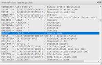
FITS Headers	Analysis > FITS Headers	analysis fitshead	In our example from earlier, where we looked at some of the different data the Chandra X-Ray Observatory collects about the light hitting the detector, such as time and energy. This data is stored in different columns of the FITS file (like in a table), where each column has a header that defines what it holds. So the time data, for example, is stored in the column with "TIME" as the header. Headers are also useful for another thing: recording outside data about the FITS file, such as who the researcher was who took the data, at what time the data was taken, what telescope took it, what object is being observed, and other documentation of the file. This analysis function displays all the headers in the FITS file. This is useful for several reasons. Most usefully, it can be useful for searching through the documentation of any FITS file for data such as that listed above. Additionally, it lists the FITS headers that can be used in the Histogram Plot analysis, although a better way to find the plottable data columns might be to look at what shows up under View > Extensions, and seeing which of the headers listed after "cols" generates a useful histogram plot.	A section of the FITS headers of Cas-A, with the object field highlighted.
Counts in Regions	Analysis > Counts in Regions Note: This is the one under the Server-side analysis heading.	analysis counts	The main purpose of this function is to count the photons (counts) in all of the regions in the image. However, it also tells you how many arcseconds are in each pixel on the image (arcseconds/pixel) which is a very useful conversion factor for getting between arcseconds and pixels. Additionally, this function give you information about the area of the region(s) you are using. This is identical to the Client-side analysis version.	Counts in Regions Analysis
Radial Profile	Analysis > Radial Profile Note: This is the one under the Server-side analysis heading.	analysis radialprofile	Radial Profile requires an annulus. This determines the flux in each region (in photons/square arcsecond) and plot the value for each region in the annulus on a graph of the surface brightness vs. the radius. This is identical to the Client-side analysis version.	Radial Profile graph. The bump in the center corresponds to the increase in brightness of the image near the bottom-left of the annulus.
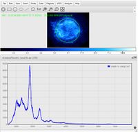
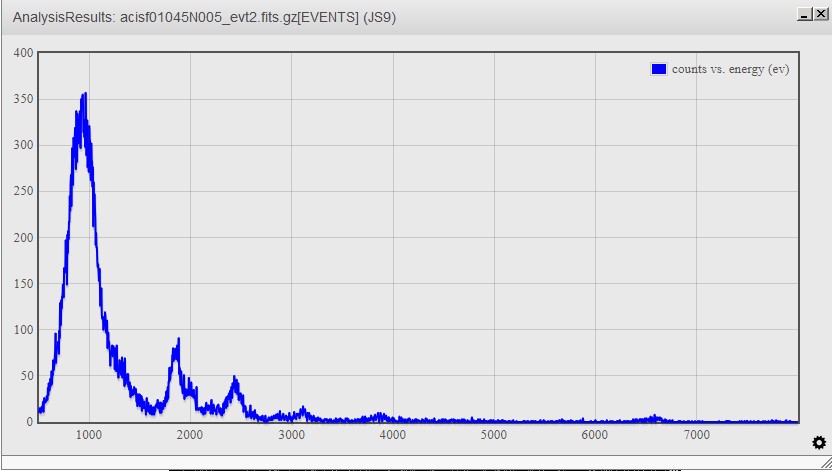
Energy Spectrum	Analysis > Energy Spectrum	analysis energyplot	This generates an energy spectrum of all regions. It displays a graph with energy (electron volts) on the x-axis and counts (photons) on the y-axis. This spectrum is extremely useful in an analysis, as it displays X-Ray spectral emission lines of the object. You can then match these spectral lines to their corresponding element (a table of some common lines can be found here) and determine what elements are present in the object. This is very useful for classifying supernovae, as each class will have some specific spectral lines that appear for the specific elements it produces.	An energy spectrum from Cas-A. Each peak is a spectral line, the tallest of which most likely corresponds to the element silicon.
Light Curve	Analysis > Light Curve Note: This is the Light Curve under the Server-side analysis heading.	analysis timeplot	This generates a light curve of all selected regions. It returns a plot display of the time (in seconds) on the x-axis and counts (photons) on the y-axis. There has also been some processing done to this plot, it is not the raw light curve. This is not the same as the light curve in NSO analysis.	The JS9 server-side light curve for Cas-A.
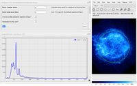
Histogram Plot	Analysis > Histogram Plot	analysis histplot	This generates a plot of a user-specified column in the FITS file of all regions. A FITS file is made up of several columns, each containing different data. To find a complete list of columns for a FITS file, go to File > display > FITS HDUs. The list item that says "EVENTS" (assuming you're using Chandra data) will have a list of cols, or columns. To generate a histogram plot, run the analysis. You should see a box. Enter the name of the column that you wish to be on the y-axis. Click "run" to generate the plot. A histogram of the "time" column will do the same thing as the Server-side analysis Light Curve function. A histogram of the "energy" column will generate an energy spectrum. The pi and pha columns will also generate an energy spectrum, although they do not contain the same scale as an energy spectrum.	A histogram plot of the pi column. The upper left hand box is where you would enter the column you would like to plot, the lower right plot is the resulting plot.
Event Filter	Analysis > Event Filter	analysis evfilter	This function will generate a new FITS file based on specified criteria. To generate the new FITS file, run the event filter analysis. You will be prompted to enter your criteria. To do this, you will have to specify a column name (see the above row for information on columns) and a range in that column to display in the format column=lower:upper. For example, pi=500:1500 will result in an image that only displays pixels that are between a pi value of 500 and 1500. You are able to analyze this image as you would any other image. You can switch back and forth between this image and the original image using the File menu. You can pair this function with the overlay function to get an image that shows different ranges in different colors.	Server-Side Analysis Example Event Filter

NSO Analysis

NSO Analysis contains analysis functions that were specifically made as an addition for the Science Olympiad version of JS9. The following analysis functions can be found in the analysis menu of JS9 under the grayed-out "NSO Analysis" Heading. Note that this will only work if you are in the Science Olympiad specific JS9. NSO Analysis is also server-side, so you will have to upload your FITS file to the remote JS9 server to use these analysis functions.

Analysis	Location in Menu	JS9 Console Command	Description/Use	Screenshots
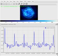
Light Curve	Analysis > Light Curve Note: This is the Light Curve under the NSO Analysis heading.	analysis lcurve	This generates a light curve of a selected region, with time on the x-axis and counts/second on the y-axis. This gives you a raw light curve of the region. This light curve can be useful to see obvious outbursts or periodicity, but tends to be more difficult to look for more subtle periodicity, which is where the next couple of NSO Analysis functions come in. Note that this is not the same light curve as the Server-side analysis version.
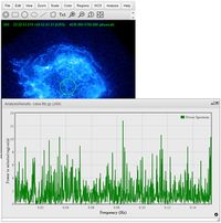
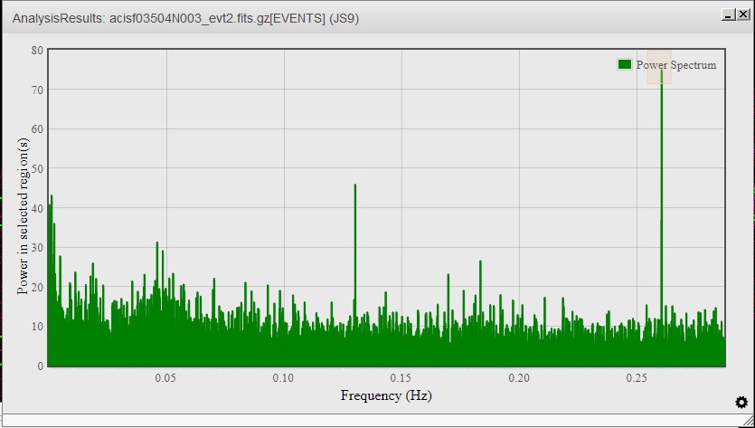
Power Spectrum	Analysis > Power Spectrum	analysis powspec	A power spectrum is a spectrum that tests waves of many different frequencies overlaid onto the light curve plot. This analysis generates a spectrum of a selected region, with the frequency of the tested wave on the x-axis and power on the (or how well it fits) y-axis. This analysis function can be very useful for determining periodicity. If the power spectrum has an obvious peak and little noise (unlike the shown period spectrum), it is likely that the period of the object is [math]\displaystyle{ \frac{1}{frequency} }[/math] in seconds. This is because Hertz is defined as [math]\displaystyle{ \frac{1}{seconds} }[/math], so flipping it would give you seconds. However, you will want to verify this period (likely using the period folding technique described below). Note that you can only run this analysis if you have already run the NSO Analysis version of Light Curve. The system generates a power spectrum essentially by overlaying a wave of different frequencies over the light curve, and then measuring how well the wave that was overlayed matches the light curve, and plotting that. The peaks show a wave frequency that appeared to fit the light curve well.	NSO Analysis Power Spectrum of Cas-A. It is fairly noisy, so there is probably no significant periodicity.
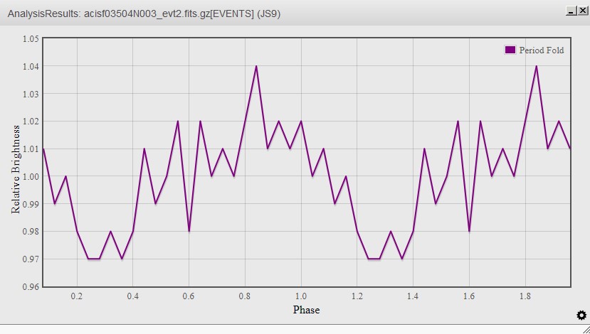
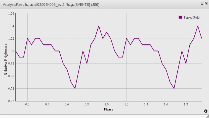
Period Folding	Analysis > Period Folding	analysis efold	This is a method of testing a potential period of a light curve of a region. It is done by taking the a certain period of a light curve and "folding" it over the rest of the light curve several times. If the period is correct, the light curve will constructively interfere and the form of the light curve will be apparent. If the period is incorrect, the light curve will destructively interfere and a periodic wave won't be apparent. This analysis requires you to enter a possible period, and it will generate a light curve of that period with the number of stacks you specify (the number of times the period is "folded"). When you run this analysis, you will be prompted to enter the period to be tested, and modify the number of stacks, if you so desire. Note that you can only run this analysis if you have already run the NSO Analysis version of Light Curve.	NSO Analysis Period Folding of Cas-A. A time of 11.79 seconds was used, obtained from finding the reciprocal of the highest-peak frequency (to get the period in seconds). A wave is seen, but it is probably not significant.
Flux in Regions	Analysis > Flux in Regions	analysis flux	This generates a window that gives you the flux in regions (in photons/arcsec2/sec). It also returns the telescope, raw counts, the raw area, the regions, and the exposure of the image.	The output of NSO Analysis Flux in Regions for Cas-A.

ImExam Plugins

Analysis done with the ImExam Plugin uses a rectangular box as a region, no matter what shape region is actually chosen. It has various analysis functions that specialize in comparing pixels in a region to one another, and has lots of visualization analysis functions. These analysis functions tend to be somewhat more unclear to work with, and probably will not be heavily emphasized in a JS9 section on an Astronomy exam.

Analysis	Location in Menu	JS9 Console Command	Description/Use	Screenshots
3dPlot	Analysis > 3dPlot	N/A	Generates a 3D Plot of the data in a region, to visualize data in a three-dimensional chart.	JS9 3dPlot of a region of Cas-A
Encircled Energy	Analysis > Encircled Energy	N/A	This generates a plot of the fraction of the total intensity of the region that has been accounted for as a function of distance from the center. In other words, as you move out from the center, what fraction of the total counts are within that radius?	JS9 Encircled Energy plot of a region of Cas-A
Histogram	Analysis > Histogram	N/A	This generates a plot of the pixels in a region that are in the same 250th percentile of their value. Note that this is not the same function as the Server-side Histogram Plot function.	An ImExam Plugin Histogram on the Cas-A image.
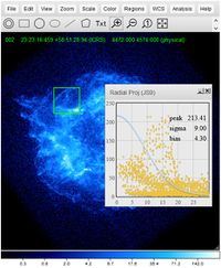
Radial Proj	Analysis > Radial Proj	N/A	This generates a scatterplot of pixel values at their respective radii. A Gaussian fit is overlaid on the scatterplot.	A plot of the radial proj for Cas-A.
Region Stats	Analysis > Region Stats	N/A	This returns the statistics of the region, including (but not limited to) the total counts, the x and y position, and width and height of the region. The region is still treated as a rectangular region for this analysis, as well.
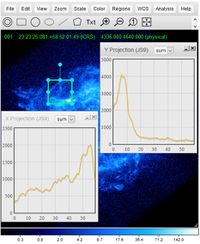
X & Y Projection	Analysis > X Projection Analysis > Y Projection	N/A	This returns the sum, average, or median (depending on which is selected) of the values of the vertical (X) or horizontal (Y) pixels along the width (X) or height (Y) of a region.	The X and Y projections of a region of Cas-A.

Sample Questions

Sample Question 1: Angular and Physical Distances

Questions like this one where you have to make angular measurements to determine physical distances are extremely common when working with JS9. This particular type of question might be worth devoting extra time to when practicing.

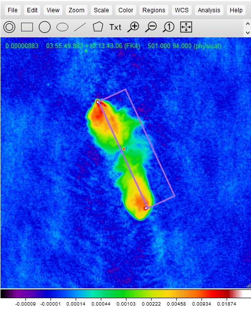
Use the JS9 “Open Remote” function to open the radio image of 3C98 using the link below. You will use a proxy server to open this image.

Data Link: http://www.jb.man.ac.uk/atlas/fits/3C98.gz

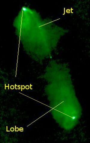
Background: This is a radio image of the radio galaxy 3C98. To complete this question, you will need to know how to identify “hotspots” in a radio galaxy. Hotspots are just the bright points at the end of the radio lobes on either end of the bright nucleus. The following image shows an example of a radio galaxy with the hotspots pointed out.

1. What is the angular separation between the two hotspots in 3C98, in arcseconds?

ExpandSolution There are several ways you can approach this one. However, because this image was not taken by Chandra, it has some weird formatting, so there is one straightforward way to go about it. Draw a rectangle between the two hotspots (I changed my colormap to sls so that the hotspots are extremely clear), similar to below. Line up the rectangle as if it were a ruler, with the two corners of one edge each touching a hotspot. Now, double-click on the rectangle to bring up the region information. The second and third text boxes show the width and height of the rectangle, respectively. In this case, we want to see how long the long end is, so that will be in the text box that corresponds to height (the box with text highlighted). Make sure FK4, FK5, or ICRS is selected in the top right corner. This is your answer. Note that the quotations in the box corresponds to the unit arcseconds. The final answer is 286.5”

2. The physical distance between these two hotspots is 193 kpc. How far away is this object, in kiloparsecs?

ExpandSolution We can plug the given distance here and the angular distance we found in the previous question into the small angle formula to determine how far away the object is. [math]\displaystyle{ \frac{\theta}{206265} = \frac{d}{D} }[/math] [math]\displaystyle{ \frac{286.5”}{206265} = \frac{193 \textrm{kpc}}{D} }[/math] 138900 kpc

Sample Question 2: X-Ray Periodicity

Use the JS9 “Open Remote” function to open the X-Ray FITS data of the neutron star 4U 1626-67 using the link below. You will use a proxy server to open this image.

Data Link: https://cxc.cfa.harvard.edu/cdaftp/science/ao04/cat4/3504/primary/acisf03504N003_evt2.fits.gz

1. What is the rotation period of this neutron star?

Expand Solution First, we need to draw the region around this neutron star. When doing this, it is important to remember that you want to select the lines extending out from the neutron star as well, shown in the image below. I used two long, rectangular regions to cover these. These extra lines are just light that was spread out from the neutron star when the instrument collected the data. You will have to zoom and pan around the image to completely surround all of them. Now, let’s find the light curve of this neutron star. Use the Analysis > Light Curve function under the NSO Analysis section to get the light curve of this object. When it loads, you find that that looks a bit like a fluffy cat tail. Not directly very useful for analysis. However, generating that light curve allows us to do something else. We can now use Analysis > Power Spectrum to help us find potential periods. When we do this, we find that there are two peaks that show potential (in the image below, the tall peak near the right of the image and the tall peak near the center). Now, let’s test them. Navigate to Analysis > Period Folding. You should see a pop-up window. Set this aside for now. To determine the value in seconds of the potential period, we need to find the frequency in the power spectrum. You can zoom in on any JS9 plot by dragging a square around where you want to zoom in. Let’s zoom in on the tallest peak to see what that one has to offer. You may have to zoom in a couple of times to get a precise enough value. I get one around 0.260585 Hz. To get the period in seconds, we need to do 1/0.260585, which gives us a period of 3.8375 seconds. Now, go back to your period folding window, and enter that value in the empty box. The resulting light curve is shown below. It looks okay, but doesn’t look amazing, don’t you agree? Maybe we ought to try that other peak to see if it yields anything better. Zoom back out of your power spectrum using the blue arrow icon in the top-left corner. Repeat the steps in the paragraph above for this peak. You should get a period of 7.675 seconds, and when plugged into the period folding window, it generates a nice light curve, shown below. Thus, we have determined a period of 7.675 seconds. Note: Differentiating between the two potential periods was difficult. The currently accepted value for this pulsar is 7.66 seconds, but the 3.84 second light curve also generated a good light curve. If in a competition, try to make your best judgment—hopefully the ES considers both possibilities to be correct.

Sample Question 3: Spectral Lines

Use the JS9 “Open Remote” function to open the X-Ray FITS data of the supernova remnant N103B using the link below. You will use a proxy server to open this image.

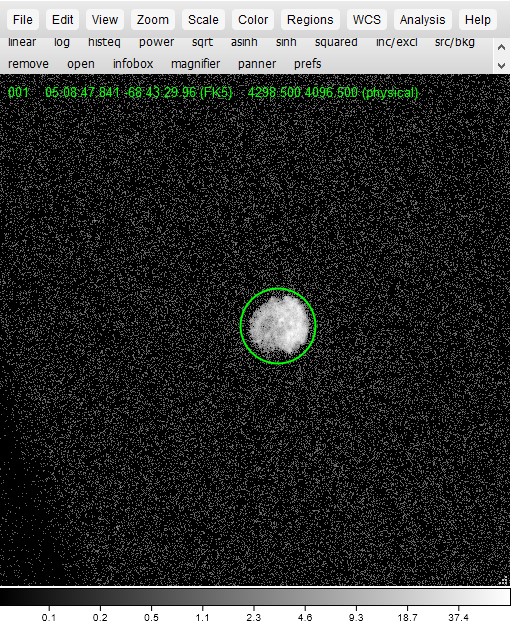
Data Link: https://cxc.cfa.harvard.edu/cdaftp/science/ao02/cat5/1045/primary/acisf01045N005_evt2.fits.gz

1. What type of supernova is this? How do you know?

Expand Solution As with the last question, the first step is to draw a region around the supernova remnant. We’ll just use a circle around it here, like so. Now, let’s use an energy spectrum to find some spectral lines. Run Analysis > Energy Spectrum. The resulting spectrum is shown below. Use the site linked at the bottom of this page (Labelled Common X-Ray Spectral Lines) to identify what elements some of these peaks correspond to. You might notice that the peak around 1850 eV corresponds to the silicon line around 1.854 keV. This is a key emission line. The other one we would look for is magnesium, which is indicative of a Type II supernova. We do not see magnesium, so we can now determine this to be Type Ia. We can determine that this is a Type Ia Supernova because it shows evidence of strong silicon emission and weak or no magnesium emission. More information on classifying supernova spectra can be found here (the formatting is awful - you have been warned).

Sample Question 4: FITS Headers

The FITS data used in Sample Questions 2 & 3 above had the same researcher carry out the observations.

1. Who was the primary researcher who took these data?

Expand Solution Any time you are asked anything about the FITS file (such as object, observer, telescope, etc.), the best thing to do is to search for it in the FITS headers. Open either of the images for question 2 or 3 and run Analysis > FITS Headers (or use File > Display > FITS Headers) and ctrl+f for the “Observer” field. We find that the observer of these images was Prof Claude Canizares.

Additional Help

The JS9 User Guide can be found under "Help" in the menu bar, in the "General Help" dropdown. Additional JS9 help can be found in the resources in this menu as well.

External Links

NSO JS9

Unofficial Chandra Archive

JS9 Guide Part I (PDF)

JS9 Guide Part II (PDF)

Common X-Ray Spectral Lines